赫尔移动平均线(Hull Moving Average,简称HMA)是一种技术指标,于2005年由Alan Hull开发。它是一种移动平均线,利用加权计算来减少滞后并提高准确性。
HMA对价格变动非常敏感,同时最大程度地减少短期波动可能产生的噪音。它通过使用加权计算来强调更近期的价格,同时平滑数据。
计算HMA的公式涉及三个步骤。首先,使用价格数据计算加权移动平均线。然后,使用第一步的结果计算第二个加权移动平均线。最后,使用第二步的结果计算第三个加权移动平均线。最终计算的结果就是移动赫尔平均线。
WMA_1 =一段时期内价格的加权移动平均值(WMA) /2
WMA_2 =价格在一段时间内的WMA
HMA_non_smooth = 2 * WMA_1 - WMA_2
HMA = HMA_non_smooth的WMA除以根号(周期)
在下面的文章中,我们将介绍如何使用Python实现HMA。本文将对计算WMA的两种方法进行详细比较。然后介绍它在时间序列建模中的作用。
Python实现HMA
方法1:将WMA计算为按时期加权的移动平均价格:
defhma(period):
wma_1=df['Adj Close'].rolling(period//2).apply(lambdax: \
np.sum(x*np.arange(1, period//2+1)) /np.sum(np.arange(1, period//2+1)), raw=True)
wma_2=df['Adj Close'].rolling(period).apply(lambdax: \
np.sum(x*np.arange(1, period+1)) /np.sum(np.arange(1, period+1)), raw=True)
diff=2*wma_1-wma_2
hma=diff.rolling(int(np.sqrt(period))).mean()
returnhma
period=20
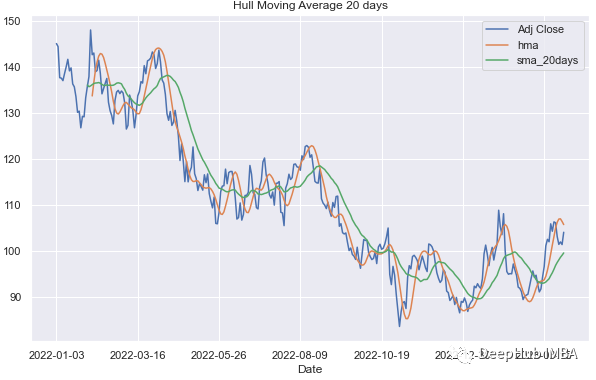
df['hma'] =hma(period)
df['sma_20days'] =df['Adj Close'].rolling(period).mean()
figsize= (10,6)
df[['Adj Close','hma','sma_20days']].plot(figsize=figsize)
plt.title('Hull Moving Average {0} days'.format(period))
plt.show()如图所示,HMA比通常的SMA反应更快:
还可以尝试更短的时间框架,看看HMA与价格曲线的关系有多密切。
 df['hma_short']=hma(14)
 df['hma_long']=hma(30)
 figsize= (12,6)
 df[['Adj Close','hma_short','hma_long']].plot(figsize=figsize)
 plt.title('Hull Moving Average')
 plt.show()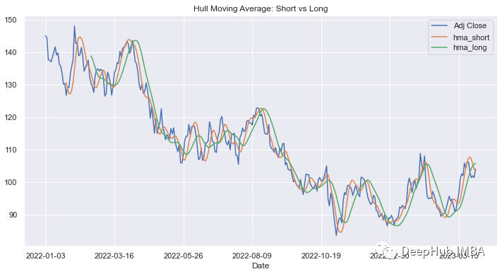
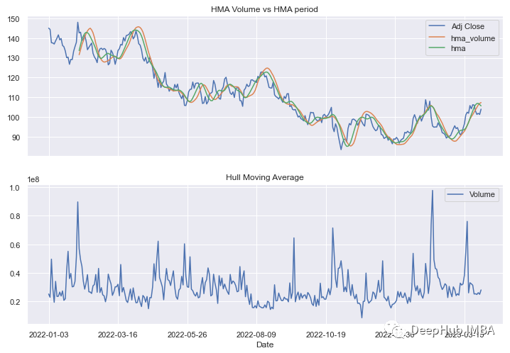
方法2,使用体量计算加权平均值:
 defhma_volume(period):
 wma_1=df['nominal'].rolling(period//2).sum()/df['Volume'].rolling(period//2).sum()
 wma_2=df['nominal'].rolling(period).sum()/df['Volume'].rolling(period).sum()
 diff=2*wma_1-wma_2
 hma=diff.rolling(int(np.sqrt(period))).mean()
 returnhma
 df['nominal'] =df['Adj Close'] *df['Volume']
 period=20
 df['hma_volume']=hma_volume(period)
 figsize=(12,8)
 fig, (ax0,ax1) =plt.subplots(nrows=2, sharex=True, subplot_kw=dict(frameon=True),figsize=figsize)
 df[['Adj Close','hma_volume','hma']].plot(ax=ax0)
 ax0.set_title('HMA Volume vs HMA period')
 df[['Volume']].plot(ax=ax1)
 ax1.set_title('Hull Moving Average')
 plt.show()
体量的HMA比第一种方法计算的HMA稍滞后:
策略的回溯测试
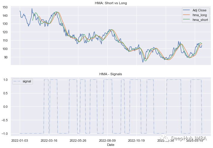
为了回测每种策略(方法1和2),我们将计算一个短期和一个长期的HMA:
当短线超过长线时,可以触发买入指令。当短线低于长线时,就会触发卖出指令。
然后我们计算每个信号产生的pnl。
方法1:
 #SIGNAL
 df['hma_short']=hma(20)
 df['hma_long']=hma(30)
 df['signal'] =np.where(df['hma_short'] >df['hma_long'],1,-1)

 #RETURN
 df['signal_shifted']=df['signal'].shift()

 ## Calculate the returns on the days we trigger a signal
 df['returns'] =df['Adj Close'].pct_change()

 ## Calculate the strategy returns
 df['strategy_returns'] =df['signal_shifted'] *df['returns']

 ## Calculate the cumulative returns
 df1=df.dropna()
 df1['cumulative_returns'] = (1+df1['strategy_returns']).cumprod()

 #PLOT
 figsize=(12,8)
 fig, (ax0,ax1) =plt.subplots(nrows=2, sharex=True, subplot_kw=dict(frameon=True),figsize=figsize)
 df[['Adj Close','hma_long','hma_short']].plot(ax=ax0)
 ax0.set_title("HMA: Short vs Long")

 df[['signal']].plot(ax=ax1,style='-.',alpha=0.4)
 ax1.legend()
 ax1.set_title("HMA - Signals")
 plt.show()

 df1['cumulative_returns'].plot(figsize=(10,4))
 plt.title("Cumulative Return")
 plt.show()
你可以看到每次产生的信号都有一条交叉线:
在数据集的整个时间段内产生的总体回报是正的,即使在某些时期它是负的:
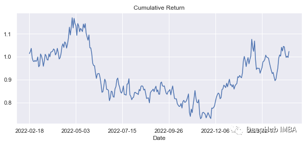
回报率:
 df1['cumulative_returns'].tail()[-1]
 #1.0229750801053696
方法2:
#SIGNAL
df['hma_volume_short']=hma_volume(20)
df['hma_volume_long']=hma_volume(30)
df['signal'] =np.where(df['hma_volume_short'] >df['hma_volume_long'],1,-1)
#RETURN
df['returns'] =df['Adj Close'].pct_change()
## Calculate the strategy returns
df['strategy_returns'] =df['signal'].shift() *df['returns']
## Calculate the cumulative returns
df2=df.dropna()
df2['cumulative_returns_volume'] = (1+df2['strategy_returns']).cumprod()
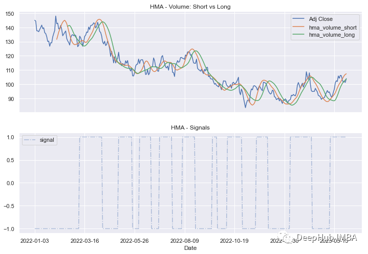
# PLOT
figsize=(12,8)
fig, (ax0,ax1) =plt.subplots(nrows=2, sharex=True, subplot_kw=dict(frameon=True),figsize=figsize)
df[['Adj Close','hma_volume_short','hma_volume_long']].plot(ax=ax0)
df[['signal']].plot(ax=ax1,style='-.',alpha=0.4)
ax0.set_title("HMA - Volume: Short vs Long")
ax1.legend()
plt.title("HMA - Signals")
plt.show()
figs= (10,4)
df2['cumulative_returns_volume'].plot(figsize=figs)
plt.title("Cumulative Return")
plt.show()看起来比第一种方法中的HMA更平滑,可以触发的信号更少(在我们的例子中只有1个):
这种策略产生的回报不是很好:0.75(0.775-1⇒-24%)
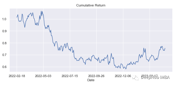
 df2['cumulative_returns_volume'].tail()[-1]
 #0.7555329108482581
我们来比较两种策略的信号:
 df['signal'] =np.where(df['hma_short'] >df['hma_long'],1,-1)
 df['signal_volume'] =np.where(df['hma_volume_short'] >df['hma_volume_long'],1,-1)
 figsize=(12,8)
 df[['signal','signal_volume']].plot(figsize=figsize)
 plt.show()
空头头寸的信号比多头头寸更多:
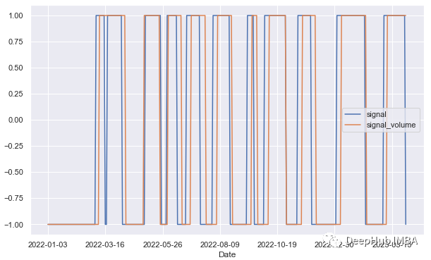
所以仅使用HMA还不足以产生有利可图的策略。我们可以使用相对强弱指数(RSI)和随机指数(Stochastic Oscillator等其他指标来确认交易信号。但是对于时间序列来说,HMA是一个很好的特征工程的方法。
HMA信号的一些解释
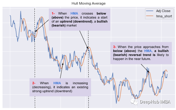
🎯交叉信号:当价格越过HMA上方时,可以解释为看涨信号,当价格越过HMA下方时,可以解释为看空信号。它也可以触发买入和卖出信号,正如我们之前已经看到的。(上图点1)。
🎯趋势跟踪信号:HMA也可用于识别趋势并生成趋势跟踪信号。当HMA倾斜向上时,它表示上升趋势,当它倾斜向下时,它表示下降趋势(上图点2)。
🎯反转信号:当价格从下方接近HMA时,看涨反转趋势可能在不久的将来发生(上图点3)。
HMA在时间序列建模的作用
HMA在时间序列建模中的作用主要是作为一个平滑滤波器,可以在一定程度上减少噪声并提高时间序列预测的准确性。在时间序列建模中,经常需要对数据进行平滑处理,以消除异常值和噪声,同时保留趋势和季节性变化的信号。HMA是一种有效的平滑滤波器,它通过加权平均的方式来计算平均值,并对较早的数据施加更大的权重,从而可以更准确地捕捉趋势性信号。
除了作为一个平滑滤波器,HMA还可以作为一个特征提取器来提取时间序列中的特征,并用于建立预测模型。例如,可以使用HMA计算时间序列中的趋势和季节性变化,并将其作为输入特征用于构建ARIMA、VAR或LSTM等预测模型。
总结
HMA不仅在交易中有广泛的应用,也是一种有用的时间序列分析工具。HMA作为一种移动平均线,可以减少时间序列中的噪声和突发性变化,从而更准确地捕捉数据的趋势性和周期性变化。在时间序列分析中,HMA通常用于平滑处理数据,以提高预测的准确性。在实际应用中,HMA常常与其他技术指标和时间序列分析方法相结合,在各种数据分析和预测任务中获取更好的预测结果。
https://avoid.overfit.cn/post/3c5f6027e1914676ad0f32c477c743c7
作者:Hanane D.