机器学习的核心目标是在未见过的新数据上实现准确预测。
当模型在训练数据上表现良好,但在测试数据上表现不佳时,即出现“过拟合”。这意味着模型从训练数据中学习了过多的噪声模式,从而丧失了在新数据上的泛化能力。
那么,过拟合的根本原因是什么?具体来说,
哪些特征(数据集的列)阻碍了模型在新数据上的有效泛化?
本文将基于实际数据集,探讨一种先进的方法来解答这一问题。
特征重要性在此场景下不再适用
如果你的第一反应是“我会查看特征重要性”,那么请重新考虑。
特征重要性无法直接反映特征在新数据上的表现。
实际上,特征重要性仅是模型在训练阶段所学内容的表现。如果模型在训练过程中学习到关于“年龄”特征的复杂模式,那么该特征的特征重要性将会很高。但这并不意味着这些模式是准确的(“准确”指的是一种具备泛化能力的模式,即在新的数据上依然成立)。
因此,我们需要采用不同的方法来解决这个问题。
案例
为了阐述该方法,我将使用一个包含 1984 年至 1988 年德国健康登记数据的数据集(该数据集可通过 Pydataset 库获得,并遵循 MIT 许可证)。
下载数据的方式非常简单:
 import pydataset
 X = pydataset.data('rwm5yr')
 y = (X['hospvis'] > 1).astype(int)
 X = X.drop('hospvis', axis = 1)
该数据集包含 19,609 行,每行记录了一名患者在特定年份的一些信息。需要注意的是,患者在不同年份都可能被观测到,因此同一患者可能出现在数据框的多行中。
目标变量是:
**hospvis**:患者在相应年份住院天数是否超过 1 天。
我们拥有 16 个特征列:
**id**:患者 ID(1-7028);**docvis**:年内就诊次数(0-121);**year**:年份(1984-1988);**edlevel**:教育水平(1-4);**age**:年龄(25-64);**outwork**:是否失业,1 表示失业,0 表示在职;**female**:性别,1 表示女性,0 表示男性;**married**:婚姻状况,1 表示已婚,0 表示未婚;**kids**:是否有子女,1 表示有,0 表示无;**hhninc**:家庭年收入(马克);**educ**:受教育年限(7-18);**self**:是否自雇,1 表示自雇,0 表示非自雇;**edlevel1**:是否为高中以下学历,1 表示是,0 表示否;**edlevel2**:是否为高中学历,1 表示是,0 表示否;**edlevel3**:是否为大学/学院学历,1 表示是,0 表示否;**edlevel4**:是否为研究生学历,1 表示是,0 表示否。
现在,将数据集划分为训练集和测试集。虽然存在更严谨的方法,如交叉验证,但为了保持简洁,我们采用简单的划分方法。但在本文中我们(简单地)将所有列视为数值特征。
 from sklearn.model_selection import train_test_split
 from catboost import CatBoostClassifier

 X_train, X_test, y_train, y_test = train_test_split(
   X, y, test_size = .2, stratify = y)

 cat = CatBoostClassifier(silent = True).fit(X_train, y_train)
模型训练完成后,我们来分析特征重要性:
 import pandas as pd

 fimpo = pd.Series(cat.feature_importances_, index = X_train.columns)
已训练模型的特征重要性。
不出所料,
docvis(就诊次数)在预测患者是否住院超过 1 天方面至关重要。
age(年龄)和
hhninc(收入)这两个特征的重要性也符合预期。但是,患者 ID(
id)的重要性排名第二则值得警惕,尤其是在我们将其视为数值特征的情况下。
接下来,计算模型在训练集和测试集上的性能指标(ROC 曲线下面积,AUC):
 from sklearn.metrics import roc_auc_score

 roc_train = roc_auc_score(y_train, cat.predict_proba(X_train)[:, 1])
 roc_test = roc_auc_score(y_test, cat.predict_proba(X_test)[:, 1])
模型在训练集和测试集上的性能。
结果显示,训练集和测试集之间的性能差距显著。这表明存在明显的过拟合现象。那么,究竟是哪些特征导致了过拟合?
什么是 SHAP 值?
我们有多种指标可以衡量模型在特定数据上的表现。但如何衡量特征在特定数据上的表现?
“SHAP 值”是解决此问题的有力工具。
通常,你可以使用专门的 Python 库来高效计算任何预测模型的 SHAP 值。但这里为了简单,我们将利用 Catboost 的原生方法:
from catboost import Pool
shap_train = pd.DataFrame(
data = cat.get_feature_importance(
data = Pool(X_train),
type = 'ShapValues')[:, :-1],
index = X_train.index,
columns = X_train.columns
)
shap_test = pd.DataFrame(
data = cat.get_feature_importance(
data = Pool(X_test),
type = 'ShapValues')[:, :-1],
index = X_test.index,
columns = X_test.columns
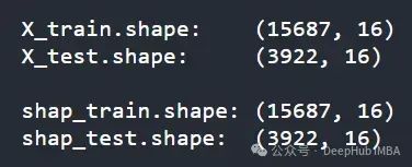
)观察
shap_train和
shap_test,你会发现它们的形状与各自的数据集相同。
SHAP 值可以量化每个特征对模型在单个或多个观测值上的最终预测的影响。
看几个例子:
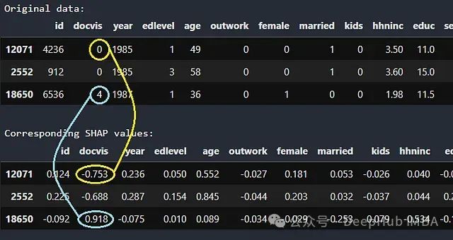
原始数据及其对应的 SHAP 值。
第 12071 行的患者就诊次数为 0,相应的 SHAP 值为-0.753,这意味着该信息将患者住院超过 1 天的概率(实际上是对数几率)降低了 0.753。相反,第 18650 行的患者就诊 4 次,这使得她住院超过 1 天的对数几率提高了 0.918。
认识 ParShap
一个特征在数据集上的性能可以通过该特征的 SHAP 值与目标变量之间的相关性来近似表示。如果模型在某个特征上学习到有效的模式,那么该特征的 SHAP 值应与目标变量高度正相关。
例如,如果我们想计算
docvis特征与测试集中观测数据的目标变量之间的相关性:
 import numpy as np

 np.corrcoef(shap_test['docvis'], y_test)
然而,SHAP 值具有可加性,即最终预测是所有特征 SHAP 值的总和。因此在计算相关性之前,先消除其他特征的影响会更有意义。这正是“偏相关”的定义。偏相关的便捷实现方式可以在 Python 库 Pingouin 中找到:
 import pingouin

 pingouin.partial_corr(
   data = pd.concat([shap_test, y_test], axis = 1).astype(float),
   x = 'docvis',
   y = y_test.name,
   x_covar = [feature for feature in shap_test.columns if feature != 'docvis']
 )
这段代码的含义是:“计算
docvis特征的 SHAP 值与测试集观测数据的目标变量之间的相关性,同时消除所有其他特征的影响。”
为了方便将此公式称为 “ParShap” (Partial correlation of Shap values,SHAP 值的偏相关)。
我们可以对训练集和测试集中的每个特征重复此过程:
 parshap_train = partial_correlation(shap_train, y_train)
 parshap_test = partial_correlation(shap_test, y_test)
注意:你可以在本文末尾找到
partial_correlation函数的定义。
现在在 x 轴上绘制
parshap_train,在 y 轴上绘制
parshap_test。
 import matplotlib.pyplot as plt

 plt.scatter(parshap_train, parshap_test)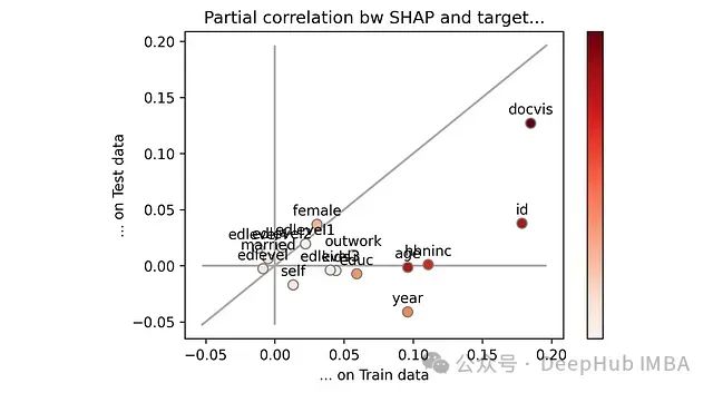
SHAP 值与目标变量的偏相关性,分别在训练集和测试集上。注意:颜色条表示特征重要性。[作者提供的图片]
如果一个特征位于对角线上,则表示它在训练集和测试集上的表现完全一致。这是理想情况,既没有过拟合也没有欠拟合。反之如果一个特征位于对角线下方,则表示它在测试集上的表现不如训练集。这属于过拟合区域。
通过视觉观察,我们可以立即发现哪些特征表现不佳:我已用蓝色圆圈标记出它们。
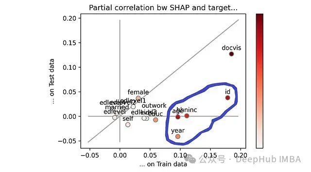
蓝色圆圈标记的特征是当前模型中最容易出现过拟合的特征。[作者提供的图片]
因此,
parshap_test和
parshap_train之间的算术差(等于每个特征与对角线之间的垂直距离)可以量化该特征对模型的过拟合程度。
parshap_diff = parshap_test - parshap_train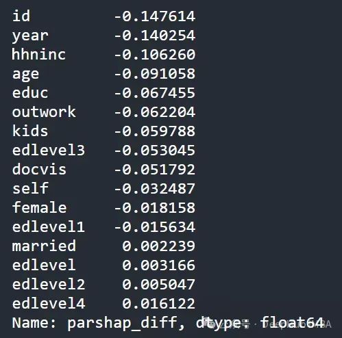
parshap_test和
parshap_train之间的算术差。[作者提供的图片]
应该如何解读这个结果?基于以上分析,该值越负,则该特征导致的过拟合程度越高。
验证
我们是否能找到一种方法来验证本文提出的观点的正确性?
从逻辑上讲,如果从数据集中移除“过拟合特征”,应该能够减少过拟合现象(即,缩小
roc_train和
roc_test之间的差距)。
因此尝试每次删除一个特征,并观察 ROC 曲线下面积的变化。
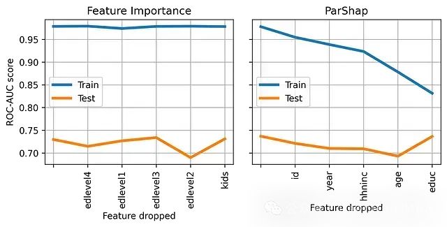
根据特征重要性(左)或 ParShap(右)排序,依次删除一个特征时,模型在训练集和测试集上的性能。
在左侧的图中,每次移除一个特征,并按照特征重要性进行排序。首先移除最不重要的特征(
edlevel4),然后移除两个最不重要的特征(
edlevel4和
edlevel1),以此类推。
在右侧的图中,执行相同的操作,但是移除的顺序由ParShap决定。首先移除 ParShap 值最小(最负)的特征(
id),然后移除两个 ParShap 值最小的特征(
id和
year),以此类推。
正如预期的那样,移除 ParShap 值最负的特征显著减少了过拟合。实际上,
roc_train的值逐渐接近
roc_test的值。
需要注意的是,这仅仅是用于验证我们推理过程的测试。通常来说,ParShap 不应被用作特征选择的方法。因为,某些特征容易出现过拟合并不意味着这些特征完全没有用处!(例如,本例中的收入和年龄)。
但是 ParShap 在为我们提供模型调试的线索方面非常有用。它可以帮助我们将注意力集中在那些需要更多特征工程或正则化的特征上。
最后以下是本文的完整,有兴趣的可以进行复现测试
本文使用的完整代码(由于随机种子,结果可能略有不同):
 ## Import libraries
 import pandas as pd
 import pydataset
 from sklearn.model_selection import train_test_split
 from catboost import CatBoostClassifier, Pool
 from sklearn.metrics import roc_auc_score
 from pingouin import partial_corr
 import matplotlib.pyplot as plt

 ## Print documentation and read data
 print('################## Print docs') ## 打印文档
 pydataset.data('rwm5yr', show_doc = True)
 X = pydataset.data('rwm5yr')
 y = (X['hospvis'] > 1).astype(int)
 X = X.drop('hospvis', axis = 1)

 ## Split data in train + test
 X_train, X_test, y_train, y_test = train_test_split(X, y, test_size = .2, stratify = y)

 ## Fit model
 cat = CatBoostClassifier(silent = True).fit(X_train, y_train)

 ## Show feature importance
 fimpo = pd.Series(cat.feature_importances_, index = X_train.columns)
 fig, ax = plt.subplots()
 fimpo.sort_values().plot.barh(ax = ax)
 fig.savefig('fimpo.png', dpi = 200, bbox_inches="tight")
 fig.show()

 ## Compute metrics
 roc_train = roc_auc_score(y_train, cat.predict_proba(X_train)[:, 1])
 roc_test = roc_auc_score(y_test, cat.predict_proba(X_test)[:, 1])
 print('\n################## Print roc') ## 打印roc
 print('roc_auc train: {:.2f}'.format(roc_train))
 print('roc_auc  test: {:.2f}'.format(roc_test))

 ## Compute SHAP values
 shap_train = pd.DataFrame(
   data = cat.get_feature_importance(data = Pool(X_train), type = 'ShapValues')[:, :-1],
   index = X_train.index,
   columns = X_train.columns
 )

 shap_test = pd.DataFrame(
   data = cat.get_feature_importance(data = Pool(X_test), type = 'ShapValues')[:, :-1],
   index = X_test.index,
   columns = X_test.columns
 )
 print('\n################## Print df shapes') ## 打印数据框的形状
 print(f'X_train.shape:    {X_train.shape}')
 print(f'X_test.shape:     {X_test.shape}\n')
 print(f'shap_train.shape: {shap_train.shape}')
 print(f'shap_test.shape:  {shap_test.shape}')

 print('\n################## Print data and SHAP') ## 打印数据和SHAP值
 print('Original data:')
 display(X_test.head(3))
 print('\nCorresponding SHAP values:')
 display(shap_test.head(3).round(3))

 ## Define function for partial correlation
 def partial_correlation(X, y):
   out = pd.Series(index = X.columns, dtype = float)
   for feature_name in X.columns:
     out[feature_name] = partial_corr(
       data = pd.concat([X, y], axis = 1).astype(float),
       x = feature_name,
       y = y.name,
       x_covar = [f for f in X.columns if f != feature_name]
     ).loc['pearson', 'r']
   return out

 ## Compute ParShap
 parshap_train = partial_correlation(shap_train, y_train)
 parshap_test = partial_correlation(shap_test, y_test)
 parshap_diff = pd.Series(parshap_test - parshap_train, name = 'parshap_diff')

 print('\n################## Print parshap_diff') ## 打印parshap差异
 print(parshap_diff.sort_values())

 ## Plot parshap
 plotmin, plotmax = min(parshap_train.min(), parshap_test.min()), max(parshap_train.max(), parshap_test.max())
 plotbuffer = .05 * (plotmax - plotmin)
 fig, ax = plt.subplots()
 if plotmin < 0:
     ax.vlines(0, plotmin - plotbuffer, plotmax + plotbuffer, color = 'darkgrey', zorder = 0)
     ax.hlines(0, plotmin - plotbuffer, plotmax + plotbuffer, color = 'darkgrey', zorder = 0)
 ax.plot(
     [plotmin - plotbuffer, plotmax + plotbuffer], [plotmin - plotbuffer, plotmax + plotbuffer],
     color = 'darkgrey', zorder = 0
 )
 sc = ax.scatter(
     parshap_train, parshap_test,
     edgecolor = 'grey', c = fimpo, s = 50, cmap = plt.cm.get_cmap('Reds'), vmin = 0, vmax = fimpo.max())
 ax.set(title = 'Partial correlation bw SHAP and target...', xlabel = '... on Train data', ylabel = '... on Test data') ## SHAP值和目标之间偏相关,在训练数据上,在测试数据上
 cbar = fig.colorbar(sc)
 cbar.set_ticks([])
 for txt in parshap_train.index:
     ax.annotate(txt, (parshap_train[txt], parshap_test[txt] + plotbuffer / 2), ha = 'center', va = 'bottom')
 fig.savefig('parshap.png', dpi = 300, bbox_inches="tight")
 fig.show()

 ## Feature selection
 n_drop_max = 5
 iterations = 4
 features = {'parshap': parshap_diff, 'fimpo': fimpo}
 features_dropped = {}
 roc_auc_scores = {
   'fimpo': {'train': pd.DataFrame(), 'test': pd.DataFrame()},
   'parshap': {'train': pd.DataFrame(), 'test': pd.DataFrame()}
 }

 for type_ in ['parshap', 'fimpo']:
   for n_drop in range(n_drop_max + 1):
     features_drop = features[type_].sort_values().head(n_drop).index.to_list()
     features_dropped[type_] = features_drop
     X_drop = X.drop(features_drop, axis = 1)
     for i in range(iterations):
       X_train, X_test, y_train, y_test = train_test_split(X_drop, y, test_size = .2, stratify = y)
       cat = CatBoostClassifier(silent = True).fit(X_train, y_train)
       roc_auc_scores[type_]['train'].loc[n_drop, i] = roc_auc_score(y_train, cat.predict_proba(X_train)[:, 1])
       roc_auc_scores[type_]['test'].loc[n_drop, i] = roc_auc_score(y_test, cat.predict_proba(X_test)[:, 1])

 ## Plot feature selection
 fig, axs = plt.subplots(1, 2, sharey = True, figsize = (8, 3))
 plt.subplots_adjust(wspace = .1)
 axs[0].plot(roc_auc_scores['fimpo']['train'].index, roc_auc_scores['fimpo']['train'].mean(axis = 1), lw = 3, label = 'Train')
 axs[0].plot(roc_auc_scores['fimpo']['test'].index, roc_auc_scores['fimpo']['test'].mean(axis = 1), lw = 3, label = 'Test')
 axs[0].set_xticks(roc_auc_scores['fimpo']['train'].index)
 axs[0].set_xticklabels([''] + features_dropped['fimpo'], rotation = 90)
 axs[0].set_title('Feature Importance') ## 特征重要性
 axs[0].set_xlabel('Feature dropped') ## 删除的特征
 axs[0].grid()
 axs[0].legend(loc = 'center left')
 axs[0].set(ylabel = 'ROC-AUC score') ## ROC-AUC分数
 axs[1].plot(roc_auc_scores['parshap']['train'].index, roc_auc_scores['parshap']['train'].mean(axis = 1), lw = 3, label = 'Train')
 axs[1].plot(roc_auc_scores['parshap']['test'].index, roc_auc_scores['parshap']['test'].mean(axis = 1), lw = 3, label = 'Test')
 axs[1].set_xticks(roc_auc_scores['parshap']['train'].index)
 axs[1].set_xticklabels([''] + features_dropped['parshap'], rotation = 90)
 axs[1].set_title('ParShap')
 axs[1].set_xlabel('Feature dropped') ## 删除的特征
 axs[1].grid()
 axs[1].legend(loc = 'center left')
 fig.savefig('feature_selection.png', dpi = 300, bbox_inches="tight")
 fig.show()
https://avoid.overfit.cn/post/47520a73a5c6469cab1116b2f036accd